Example search for a solution. Blue lines show constraints, red points show iterated solutions.

Interior-point methods (also referred to as barrier methods or IPMs) are algorithms for solving linear and non-linear convex optimization problems. IPMs combine two advantages of previously-known algorithms:

• Theoretically, their run-time is polynomial—in contrast to the simplex method, which has exponential run-time in the worst case.
• Practically, they run as fast as the simplex method—in contrast to the ellipsoid method, which has polynomial run-time in theory but is very slow in practice.

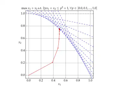
In contrast to the simplex method which traverses the boundary of the feasible region, and the ellipsoid method which bounds the feasible region from outside, an IPM reaches a best solution by traversing the interior of the feasible region—hence the name.

History

An interior point method was discovered by Soviet mathematician I. I. Dikin in 1967.^[1] The method was reinvented in the U.S. in the mid-1980s. In 1984, Narendra Karmarkar developed a method for linear programming called Karmarkar's algorithm,^[2] which runs in provably polynomial time (${\displaystyle O(n^{3.5}L)}$ operations on L-bit numbers, where n is the number of variables and constants), and is also very efficient in practice. Karmarkar's paper created a surge of interest in interior point methods. Two years later, James Renegar invented the first path-following interior-point method, with run-time ${\displaystyle O(n^{3}L)}$. The method was later extended from linear to convex optimization problems, based on a self-concordant barrier function used to encode the convex set.^[3]

Any convex optimization problem can be transformed into minimizing (or maximizing) a linear function over a convex set by converting to the epigraph form.^[4] The idea of encoding the feasible set using a barrier and designing barrier methods was studied by Anthony V. Fiacco, Garth P. McCormick, and others in the early 1960s. These ideas were mainly developed for general nonlinear programming, but they were later abandoned due to the presence of more competitive methods for this class of problems (e.g. sequential quadratic programming).

Yurii Nesterov and Arkadi Nemirovski came up with a special class of such barriers that can be used to encode any convex set. They guarantee that the number of iterations of the algorithm is bounded by a polynomial in the dimension and accuracy of the solution.^[5][3]

The class of primal-dual path-following interior-point methods is considered the most successful. Mehrotra's predictor–corrector algorithm provides the basis for most implementations of this class of methods.^[6]

Definitions

We are given a convex program of the form:

$${\displaystyle {\begin{aligned}{\underset {x\in \mathbb {R} ^{n}}{\text{minimize}}}\quad &f(x)\\{\text{subject to}}\quad &g_{i}(x)\leq 0{\text{ for }}i=1,\dots ,m,\\&x\in G.\end{aligned}}}$$

where f and the g_i are convex functions and G is a convex set. Without loss of generality, we can assume that the objective f is a linear function. We assume that the constraint functions belong to some family (e.g. quadratic functions), so that the program can be represented by a finite vector of coefficients (e.g. the coefficients to the quadratic functions). The dimension of this coefficient vector is called the size of the program. A numerical solver for a given family of programs is an algorithm that, given the coefficient vector, generates a sequence of approximate solutions x_t for t=1,2,..., using finitely many arithmetic operations. A numerical solver is called convergent if, for any progarm from the family and any positive ε>0, there is some T (which may depend on the program and on ε) such that, for any t>T, the approximate solution x_t is ε-approximate, that is:

f(x) - f^* ≤ ε

g_i(x) ≤ ε for i in 1,...,m,

x in G,

where f^* is the optimal solution. A solver is called polynomial if the total number of arithmetic operations in the first T steps is at most

poly(problem-size) * log(V/ε),

where V represents e.g. the largest value in the coefficient vector. In other words, V/ε is the "relative accuracy" of the solution - the accuracy w.r.t. the largest coefficient. log(V/ε) represents the number of "accuracy digits". Therefore, a solver is 'polynomial' if each additional digit of accuracy requires a number of operations that is polynomial in the problem size.

Types

Types of interior point methods include:

• Potential reduction methods: Karmarkar's algorithm was the first one.
• Path-following methods: the algorithms of James Renegar^[7] and Clovis Gonzaga^[8] were the first ones.
• Primal-dual methods.

Path-following methods

Potential-reduction methods

Potential-reduction methods are elaborated in.^[3]: Sec.5 For potential-reduction methods, the problem is presented in the conic form:

minimize c^Tx s.t. x in {b+L} ᚢ K,

where b is a vector in Rⁿ, L is a linear subspace in Rⁿ (so b+L is an affine plane), and K is a closed pointed convex cone with a nonempty interior. Every convex program can be converted to the conic form.

Primal-dual methods

The primal-dual method's idea is easy to demonstrate for constrained nonlinear optimization.^[9][10] For simplicity, consider the following nonlinear optimization problem with inequality constraints:

${\displaystyle {\begin{aligned}\operatorname {minimize} \quad &f(x)\\{\text{subject to}}\quad &x\in \mathbb {R} ^{n},\\&c_{i}(x)\geq 0{\text{ for }}i=1,\ldots ,m,\\{\text{where}}\quad &f:\mathbb {R} ^{n}\to \mathbb {R} ,\ c_{i}:\mathbb {R} ^{n}\to \mathbb {R} .\end{aligned}}\quad (1)}$

This inequality-constrained optimization problem is solved by converting it into an unconstrained objective function whose minimum we hope to find efficiently. Specifically, the logarithmic barrier function associated with (1) is

${\displaystyle B(x,\mu )=f(x)-\mu \sum _{i=1}^{m}\log(c_{i}(x)).\quad (2)}$

Here ${\displaystyle \mu }$ is a small positive scalar, sometimes called the "barrier parameter". As ${\displaystyle \mu }$ converges to zero the minimum of ${\displaystyle B(x,\mu )}$ should converge to a solution of (1).

The gradient of a differentiable function ${\displaystyle h:\mathbb {R} ^{n}\to \mathbb {R} }$ is denoted ${\displaystyle \nabla h}$. The gradient of the barrier function is

${\displaystyle \nabla B(x,\mu )=\nabla f(x)-\mu \sum _{i=1}^{m}{\frac {1}{c_{i}(x)}}\nabla c_{i}(x).\quad (3)}$

In addition to the original ("primal") variable ${\displaystyle x}$ we introduce a Lagrange multiplier-inspired dual variable ${\displaystyle \lambda \in \mathbb {R} ^{m}}$

${\displaystyle c_{i}(x)\lambda _{i}=\mu ,\quad \forall i=1,\ldots ,m.\quad (4)}$

Equation (4) is sometimes called the "perturbed complementarity" condition, for its resemblance to "complementary slackness" in KKT conditions.

We try to find those ${\displaystyle (x_{\mu },\lambda _{\mu })}$ for which the gradient of the barrier function is zero.

Substituting ${\displaystyle 1/c_{i}(x)=\lambda _{i}/\mu }$ from (4) into (3), we get an equation for the gradient:

${\displaystyle \nabla B(x_{\mu },\lambda _{\mu })=\nabla f(x_{\mu })-J(x_{\mu })^{T}\lambda _{\mu }=0,\quad (5)}$

where the matrix ${\displaystyle J}$ is the Jacobian of the constraints ${\displaystyle c(x)}$.

The intuition behind (5) is that the gradient of ${\displaystyle f(x)}$ should lie in the subspace spanned by the constraints' gradients. The "perturbed complementarity" with small ${\displaystyle \mu }$ (4) can be understood as the condition that the solution should either lie near the boundary ${\displaystyle c_{i}(x)=0}$, or that the projection of the gradient ${\displaystyle \nabla f}$ on the constraint component ${\displaystyle c_{i}(x)}$ normal should be almost zero.

Let ${\displaystyle (p_{x},p_{\lambda })}$ be the search direction for iteratively updating ${\displaystyle (x,\lambda )}$. Applying Newton's method to (4) and (5), we get an equation for ${\displaystyle (p_{x},p_{\lambda })}$:

${\displaystyle {\begin{pmatrix}H(x,\lambda )&-J(x)^{T}\\\operatorname {diag} (\lambda )J(x)&\operatorname {diag} (c(x))\end{pmatrix}}{\begin{pmatrix}p_{x}\\p_{\lambda }\end{pmatrix}}={\begin{pmatrix}-\nabla f(x)+J(x)^{T}\lambda \\\mu 1-\operatorname {diag} (c(x))\lambda \end{pmatrix}},}$

where ${\displaystyle H}$ is the Hessian matrix of ${\displaystyle B(x,\mu )}$, ${\displaystyle \operatorname {diag} (\lambda )}$ is a diagonal matrix of ${\displaystyle \lambda }$, and ${\displaystyle \operatorname {diag} (c(x))}$ is the diagonal matrix of ${\displaystyle c(x)}$.

Because of (1), (4) the condition

${\displaystyle \lambda \geq 0}$

should be enforced at each step. This can be done by choosing appropriate ${\displaystyle \alpha }$:

${\displaystyle (x,\lambda )\to (x+\alpha p_{x},\lambda +\alpha p_{\lambda }).}$

Special cases

Here are some special cases of convex programs, that can be solved efficiently by interior-point methods.^{[3]: Sec.10}

• Linear programming: given a program of the form: minimize c^Tx s.t. Ax ≤ b, we can apply path-following methods with the barrier ${\displaystyle b(x):=-\sum _{j=1}^{m}\ln(b_{j}-a_{j}^{T}x)}$. It is a self-concordant barrier with parameter M=m (the number of constraints). Therefore, the number of required Newtoמ steps for the path-following method is O(mn²), and the total runtime complexity is O(m^3/2 n²).
• Quadratically constrained quadratic programing: given a program of the form: minimize d^Tx s.t. f_j(x) := x^T A_j x + b_j^Tx + c_j ≤ 0 for all j in 1,...,m, where all matrices A_j are positive-semidefinite, we can apply path-following methods with the barrier ${\displaystyle b(x):=-\sum _{j=1}^{m}\ln(-f_{j}(x))}$. It is a self-concordant barrier with parameter M=m. The Newton complexity is O((m+n)n²), and the total runtime complexity is O(m^1/2 (m+n) n²).
• Approximation in L_p norm: we are given a problem of the form minimize sum_j |v_j-u_j^Tx|^p, where 1<p<∞, u_j are vectors and v_j are scalars. After converting to the standard form, we can apply path-following methods with a self-concordant barrier with parameter M=4m. The Newton complexity is O((m+n)n²), and the total runtime complexity is O(m^1/2 (m+n) n²).
• Geometric programming: we are given a problem with objective function f₀(x)=sum_i c_i0 exp(a_i^Tx), and constraints f_j(x)=sum_i c_ij exp(a_i^Tx) ≤ d_j for j in 1,...,m and i in 1,...,k. There is a self-concordant barrier with parameter 2k+m. The path-following method has Newton complexity O(mk²+k³+n³) and total complexity O((k+m)^1/2[mk²+k³+n³]).
• Semidefinite programming.^{[3]: Sec.11}

See also

• Affine scaling
• Augmented Lagrangian method
• Chambolle-Pock algorithm
• Karush–Kuhn–Tucker conditions
• Penalty method

References

• Bonnans, J. Frédéric; Gilbert, J. Charles; Lemaréchal, Claude; Sagastizábal, Claudia A. (2006). Numerical optimization: Theoretical and practical aspects. Universitext (Second revised ed. of translation of 1997 French ed.). Berlin: Springer-Verlag. pp. xiv+490. doi:10.1007/978-3-540-35447-5. ISBN 978-3-540-35445-1. MR 2265882.
• Nocedal, Jorge; Stephen Wright (1999). Numerical Optimization. New York, NY: Springer. ISBN 978-0-387-98793-4.
• Press, WH; Teukolsky, SA; Vetterling, WT; Flannery, BP (2007). "Section 10.11. Linear Programming: Interior-Point Methods". Numerical Recipes: The Art of Scientific Computing (3rd ed.). New York: Cambridge University Press. ISBN 978-0-521-88068-8.

References

- ↑ Dikin, I.I. (1967). "Iterative solution of problems of linear and quadratic programming". Dokl. Akad. Nauk SSSR. 174 (1): 747–748.
- ↑ Karmarkar, N. (1984). "A new polynomial-time algorithm for linear programming" (PDF). Proceedings of the sixteenth annual ACM symposium on Theory of computing – STOC '84. p. 302. doi:10.1145/800057.808695. ISBN 0-89791-133-4. Archived from the original (PDF) on 28 December 2013.
- 1 2 3 4 5 6 7 8 9 10 11 12 Arkadi Nemirovsky (2004). Interior point polynomial-time methods in convex programming.
- ↑ Boyd, Stephen; Vandenberghe, Lieven (2004). Convex Optimization. Cambridge: Cambridge University Press. p. 143. ISBN 978-0-521-83378-3. MR 2061575.
- ↑ Wright, Margaret H. (2004). "The interior-point revolution in optimization: History, recent developments, and lasting consequences". Bulletin of the American Mathematical Society. 42: 39–57. doi:10.1090/S0273-0979-04-01040-7. MR 2115066.
- ↑ Potra, Florian A.; Stephen J. Wright (2000). "Interior-point methods". Journal of Computational and Applied Mathematics. 124 (1–2): 281–302. doi:10.1016/S0377-0427(00)00433-7.
- 1 2 Renegar, James (1 January 1988). "A polynomial-time algorithm, based on Newton's method, for linear programming". Mathematical Programming. 40 (1): 59–93. doi:10.1007/BF01580724. ISSN 1436-4646.
- 1 2 Gonzaga, Clovis C. (1989), Megiddo, Nimrod (ed.), "An Algorithm for Solving Linear Programming Problems in O(n3L) Operations", Progress in Mathematical Programming: Interior-Point and Related Methods, New York, NY: Springer, pp. 1–28, doi:10.1007/978-1-4613-9617-8_1, ISBN 978-1-4613-9617-8, retrieved 22 November 2023
- ↑ Mehrotra, Sanjay (1992). "On the Implementation of a Primal-Dual Interior Point Method". SIAM Journal on Optimization. 2 (4): 575–601. doi:10.1137/0802028.
- ↑ Wright, Stephen (1997). Primal-Dual Interior-Point Methods. Philadelphia, PA: SIAM. ISBN 978-0-89871-382-4.